Compute an aggregation rule
Source:R/mixture.R, R/print-mixture.R, R/summary-mixture.R
mixture-opera.RdThe function mixture builds an
aggregation rule chosen by the user.
It can then be used to predict new observations Y sequentially.
If observations Y and expert advice experts are provided,
mixture is trained by predicting the observations in Y
sequentially with the help of the expert advice in experts.
At each time instance \(t=1,2,\dots,T\), the mixture forms a prediction of Y[t,] by assigning
a weight to each expert and by combining the expert advice.
Arguments
- Y
A matrix with T rows and d columns. Each row
Y[t,]contains a d-dimensional observation to be predicted sequentially.- experts
An array of dimension
c(T,d,K), whereTis the length of the data-set,dthe dimension of the observations, andKis the number of experts. It contains the expert forecasts. Each vectorexperts[t,,k]corresponds to the d-dimensional prediction ofY[t,]proposed by expert k at time \(t=1,\dots,T\). In the case of real prediction (i.e., \(d = 1\)),expertsis a matrix withTrows andKcolumns.- model
A character string specifying the aggregation rule to use. Currently available aggregation rules are:
- 'EWA'
Exponentially weighted average aggregation rules (Cesa-Bianchi and Lugosi 2006) . A positive learning rate eta can be chosen by the user. The bigger it is the faster the aggregation rule will learn from observations and experts performances. However, too high values lead to unstable weight vectors and thus unstable predictions. If it is not specified, the learning rate is calibrated online. A finite grid of potential learning rates to be optimized online can be specified with grid.eta.
- 'FS'
Fixed-share aggregation rule (Cesa-Bianchi and Lugosi 2006) . As for
ewa, a learning rate eta can be chosen by the user or calibrated online. The main difference withewaaggregation rule rely in the mixing rate alpha\(\in [0,1]\) which considers at each instance a small probabilityalphato have a rupture in the sequence and that the best expert may change. Fixed-share aggregation rule can thus compete with the best sequence of experts that can change a few times (seeoracle), whileewacan only compete with the best fixed expert. The mixing rate alpha is either chosen by the user either calibrated online. Finite grids of learning rates and mixing rates to be optimized can be specified with parameters grid.eta and grid.alpha.- 'Ridge'
Online Ridge regression (Cesa-Bianchi and Lugosi 2006) . It minimizes at each instance a penalized criterion. It forms at each instance linear combination of the experts' forecasts and can assign negative weights that not necessarily sum to one. It is useful if the experts are biased or correlated. It cannot be used with specialized experts. A positive regularization coefficient lambda can either be chosen by the user or calibrated online. A finite grid of coefficient to be optimized can be specified with a parameter grid.lambda.
- 'MLpol', 'MLewa', 'MLprod'
Aggregation rules with multiple learning rates that are theoretically calibrated (Gaillard et al. 2014) .
- 'BOA'
Bernstein online Aggregation (Wintenberger 2017) . The learning rates are automatically calibrated.
- 'OGD'
Online Gradient descent (Zinkevich 2003) . See also (Hazan 2019) . The optimization is performed with a time-varying learning rate. At time step \(t \geq 1\), the learning rate is chosen to be \(t^{-\alpha}\), where \(\alpha\) is provided by alpha in the parameters argument. The algorithm may or not perform a projection step into the simplex space (non-negative weights that sum to one) according to the value of the parameter 'simplex' provided by the user.
- 'FTRL'
Follow The Regularized Leader (Shalev-Shwartz and Singer 2007) . Note that here, the linearized version of FTRL is implemented (see Chap. 5 of (Hazan 2019) ).
FTRLis the online counterpart of empirical risk minimization. It is a family of aggregation rules (including OGD) that uses at any time the empirical risk minimizer so far with an additional regularization. The online optimization can be performed on any bounded convex set that can be expressed with equality or inequality constraints. Note that this method is still under development and a beta version.The user must provide (in the parameters's list):
- 'eta'
The learning rate.
- 'fun_reg'
The regularization function to be applied on the weigths. See
auglag: fn.- 'constr_eq'
The equality constraints (e.g. sum(w) = 1). See
auglag: heq.- 'constr_ineq'
The inequality constraints (e.g. w > 0). See
auglag: hin.- 'fun_reg_grad'
(optional) The gradient of the regularization function. See
auglag: gr.- 'constr_eq_jac'
(optional) The Jacobian of the equality constraints. See
auglag: heq.jac- 'constr_ineq_jac'
(optional) The Jacobian of the inequality constraints. See
auglag: hin.jac
or set default to TRUE. In the latter, FTRL is performed with Kullback regularization (
fun_reg(x) = sum(x log (x/w0))on the simplex (constr_eq(w) = sum(w) - 1andconstr_ineq(w) = w). Parameters w0 (weight initialization), and max_iter can also be provided.
- loss.type
character, list, or function("square").- character
Name of the loss to be applied ('square', 'absolute', 'percentage', or 'pinball');
- list
List with field
nameequal to the loss name. If using pinball loss, fieldtauequal to the required quantile in [0,1];- function
A custom loss as a function of two parameters (prediction, observation). For example, $f(x,y) = abs(x-y)/y$ for the Mean absolute percentage error or $f(x,y) = (x-y)^2$ for the squared loss.
- loss.gradient
boolean, function(TRUE).- boolean
If TRUE, the aggregation rule will not be directly applied to the loss function at hand, but to a gradient version of it. The aggregation rule is then similar to gradient descent aggregation rule.
- function
Can be provided if loss.type is a function. It should then be a sub-derivative of the loss in its first component (i.e., in the prediction). For instance, $g(x) = (x-y)$ for the squared loss.
- coefficients
A probability vector of length K containing the prior weights of the experts (not possible for 'MLpol'). The weights must be non-negative and sum to 1.
- awake
A matrix specifying the activation coefficients of the experts. Its entries lie in
[0,1]. Possible if some experts are specialists and do not always form and suggest prediction. If the expert numberkat instancetdoes not form any prediction of observationY_t, we can putawake[t,k]=0so that the mixture does not consider expertkin the mixture to predictY_t.- parameters
A list that contains optional parameters for the aggregation rule. If no parameters are provided, the aggregation rule is fully calibrated online. Possible parameters are:
- eta
A positive number defining the learning rate. Possible if model is either 'EWA' or 'FS'
- grid.eta
A vector of positive numbers defining potential learning rates for 'EWA' of 'FS'. The learning rate is then calibrated by sequentially optimizing the parameter in the grid. The grid may be extended online if needed by the aggregation rule.
- gamma
A positive number defining the exponential step of extension of grid.eta when it is needed. The default value is 2.
- alpha
A number in [0,1]. If the model is 'FS', it defines the mixing rate. If the model is 'OGD', it defines the order of the learning rate: \(\eta_t = t^{-\alpha}\).
- grid.alpha
A vector of numbers in [0,1] defining potential mixing rates for 'FS' to be optimized online. The grid is fixed over time. The default value is
[0.0001,0.001,0.01,0.1].- lambda
A positive number defining the smoothing parameter of 'Ridge' aggregation rule.
- grid.lambda
Similar to
grid.etafor the parameterlambda.- simplex
A boolean that specifies if 'OGD' does a project on the simplex. In other words, if TRUE (default) the online gradient descent will be under the constraint that the weights sum to 1 and are non-negative. If FALSE, 'OGD' performs an online gradient descent on K dimensional real space. without any projection step.
- averaged
A boolean (default is FALSE). If TRUE the coefficients and the weights returned (and used to form the predictions) are averaged over the past. It leads to more stability on the time evolution of the weights but needs more regularity assumption on the underlying process generating the data (i.i.d. for instance).
- quiet
boolean. Whether or not to display progress bars.- ...
Additional parameters
- x
An object of class mixture
- object
An object of class mixture
Value
An object of class mixture that can be used to perform new predictions.
It contains the parameters model, loss.type, loss.gradient,
experts, Y, awake, and the fields
- coefficients
A vector of coefficients assigned to each expert to perform the next prediction.
- weights
A matrix of dimension
c(T,K), withTthe number of instances to be predicted andKthe number of experts. Each row contains the convex combination to form the predictions.- prediction
A matrix with
Trows anddcolumns that contains the predictions outputted by the aggregation rule.- loss
The average loss (as stated by parameter
loss.type) suffered by the aggregation rule.- parameters
The learning parameters chosen by the aggregation rule or by the user.
- training
A list that contains useful temporary information of the aggregation rule to be updated and to perform predictions.
References
Cesa-Bianchi N, Lugosi G (2006).
Prediction, learning, and games.
Cambridge university press.
Gaillard P, Stoltz G, van Erven T (2014).
“A Second-order Bound with Excess Losses.”
In Proceedings of COLT'14, volume 35, 176–196.
Hazan E (2019).
“Introduction to online convex optimization.”
arXiv preprint arXiv:1909.05207.
Shalev-Shwartz S, Singer Y (2007).
“A primal-dual perspective of online learning algorithms.”
Machine Learning, 69(2), 115–142.
Wintenberger O (2017).
“Optimal learning with Bernstein online aggregation.”
Machine Learning, 106(1), 119–141.
Zinkevich M (2003).
“Online convex programming and generalized infinitesimal gradient ascent.”
In Proceedings of the 20th international conference on machine learning (icml-03), 928–936.
See also
See opera-package and opera-vignette for a brief example about how to use the package.
Examples
library('opera') # load the package
set.seed(1)
# Example: find the best one week ahead forecasting strategy (weekly data)
# packages
library(mgcv)
#> Loading required package: nlme
#> This is mgcv 1.9-3. For overview type 'help("mgcv-package")'.
# import data
data(electric_load)
idx_data_test <- 620:nrow(electric_load)
data_train <- electric_load[-idx_data_test, ]
data_test <- electric_load[idx_data_test, ]
# Build the expert forecasts
# ##########################
# 1) A generalized additive model
gam.fit <- gam(Load ~ s(IPI) + s(Temp) + s(Time, k=3) +
s(Load1) + as.factor(NumWeek), data = data_train)
gam.forecast <- predict(gam.fit, newdata = data_test)
# 2) An online autoregressive model on the residuals of a medium term model
# Medium term model to remove trend and seasonality (using generalized additive model)
detrend.fit <- gam(Load ~ s(Time,k=3) + s(NumWeek) + s(Temp) + s(IPI), data = data_train)
electric_load$Trend <- c(predict(detrend.fit), predict(detrend.fit,newdata = data_test))
electric_load$Load.detrend <- electric_load$Load - electric_load$Trend
# Residual analysis
ar.forecast <- numeric(length(idx_data_test))
for (i in seq(idx_data_test)) {
ar.fit <- ar(electric_load$Load.detrend[1:(idx_data_test[i] - 1)])
ar.forecast[i] <- as.numeric(predict(ar.fit)$pred) + electric_load$Trend[idx_data_test[i]]
}
# Aggregation of experts
###########################
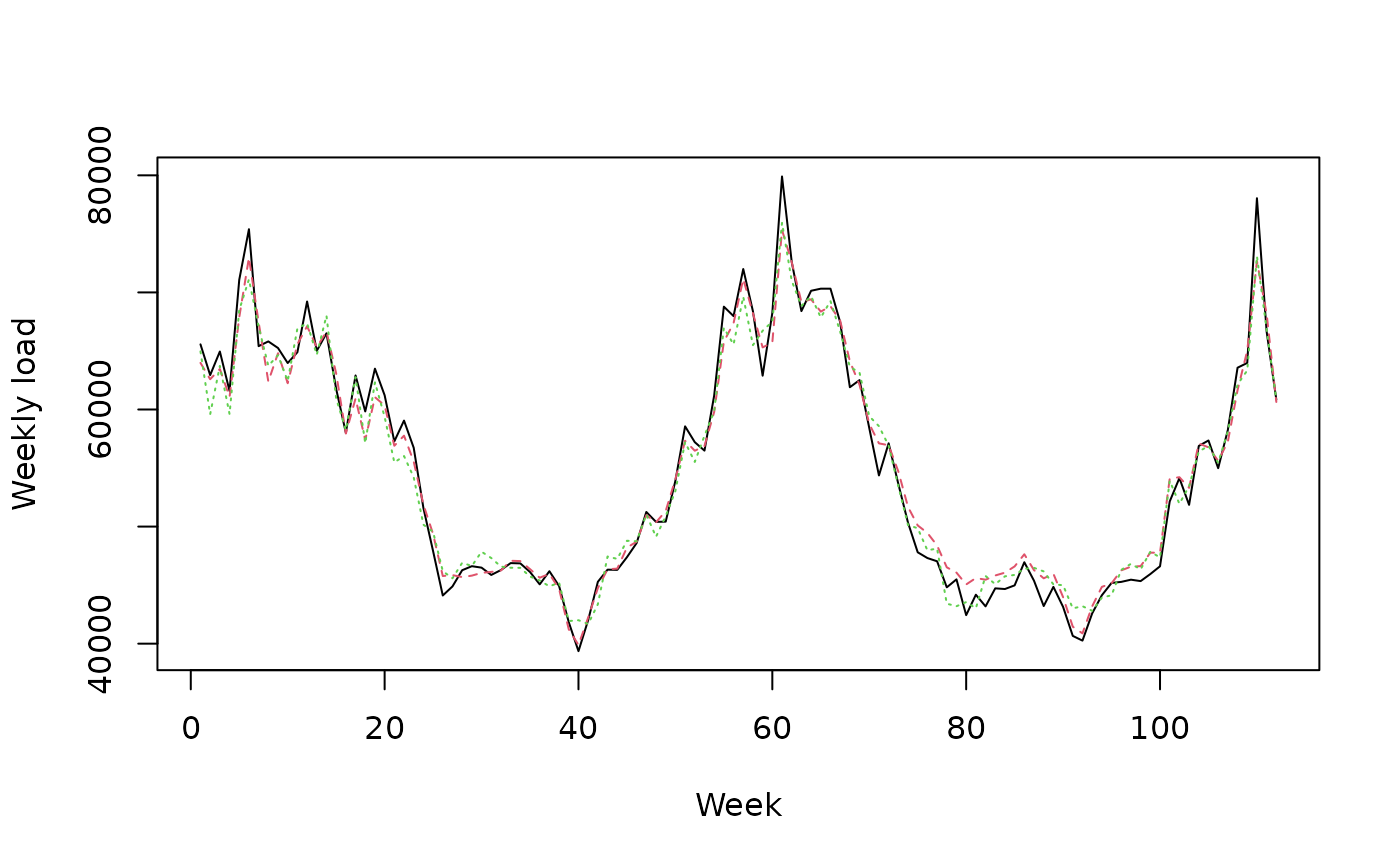
X <- cbind(gam.forecast, ar.forecast)
colnames(X) <- c('gam', 'ar')
Y <- data_test$Load
matplot(cbind(Y, X), type = 'l', col = 1:6, ylab = 'Weekly load', xlab = 'Week')
 # How good are the expert? Look at the oracles
oracle.convex <- oracle(Y = Y, experts = X, loss.type = 'square', model = 'convex')
if(interactive()){
plot(oracle.convex)
}
oracle.convex
#> Call:
#> oracle.default(Y = Y, experts = X, model = "convex", loss.type = "square")
#>
#> Coefficients:
#> gam ar
#> 0.751 0.249
#>
#> rmse mape
#> Best expert oracle: 1480 0.0202
#> Uniform combination: 1480 0.0206
#> Best convex oracle: 1450 0.0200
# Is a single expert the best over time ? Are there breaks ?
oracle.shift <- oracle(Y = Y, experts = X, loss.type = 'percentage', model = 'shifting')
if(interactive()){
plot(oracle.shift)
}
oracle.shift
#> Call:
#> oracle.default(Y = Y, experts = X, model = "shifting", loss.type = "percentage")
#>
#> 0 shifts 28 shifts 55 shifts 83 shifts 111 shifts
#> mape: 0.0202 0.0159 0.0154 0.0154 0.0154
# Online aggregation of the experts with BOA
#############################################
# Initialize the aggregation rule
m0.BOA <- mixture(model = 'BOA', loss.type = 'square')
# Perform online prediction using BOA There are 3 equivalent possibilities 1)
# start with an empty model and update the model sequentially
m1.BOA <- m0.BOA
for (i in 1:length(Y)) {
m1.BOA <- predict(m1.BOA, newexperts = X[i, ], newY = Y[i], quiet = TRUE)
}
# 2) perform online prediction directly from the empty model
m2.BOA <- predict(m0.BOA, newexpert = X, newY = Y, online = TRUE, quiet = TRUE)
# 3) perform the online aggregation directly
m3.BOA <- mixture(Y = Y, experts = X, model = 'BOA', loss.type = 'square', quiet = TRUE)
# These predictions are equivalent:
identical(m1.BOA, m2.BOA) # TRUE
#> [1] TRUE
identical(m1.BOA, m3.BOA) # TRUE
#> [1] TRUE
# Display the results
summary(m3.BOA)
#> Aggregation rule: BOA
#> Loss function: squareloss
#> Gradient trick: TRUE
#> Coefficients:
#> gam ar
#> 0.738 0.262
#>
#> Number of experts: 2
#> Number of observations: 112
#> Dimension of the data: 1
#>
#> rmse mape
#> BOA 1490 0.0203
#> Uniform 1480 0.0206
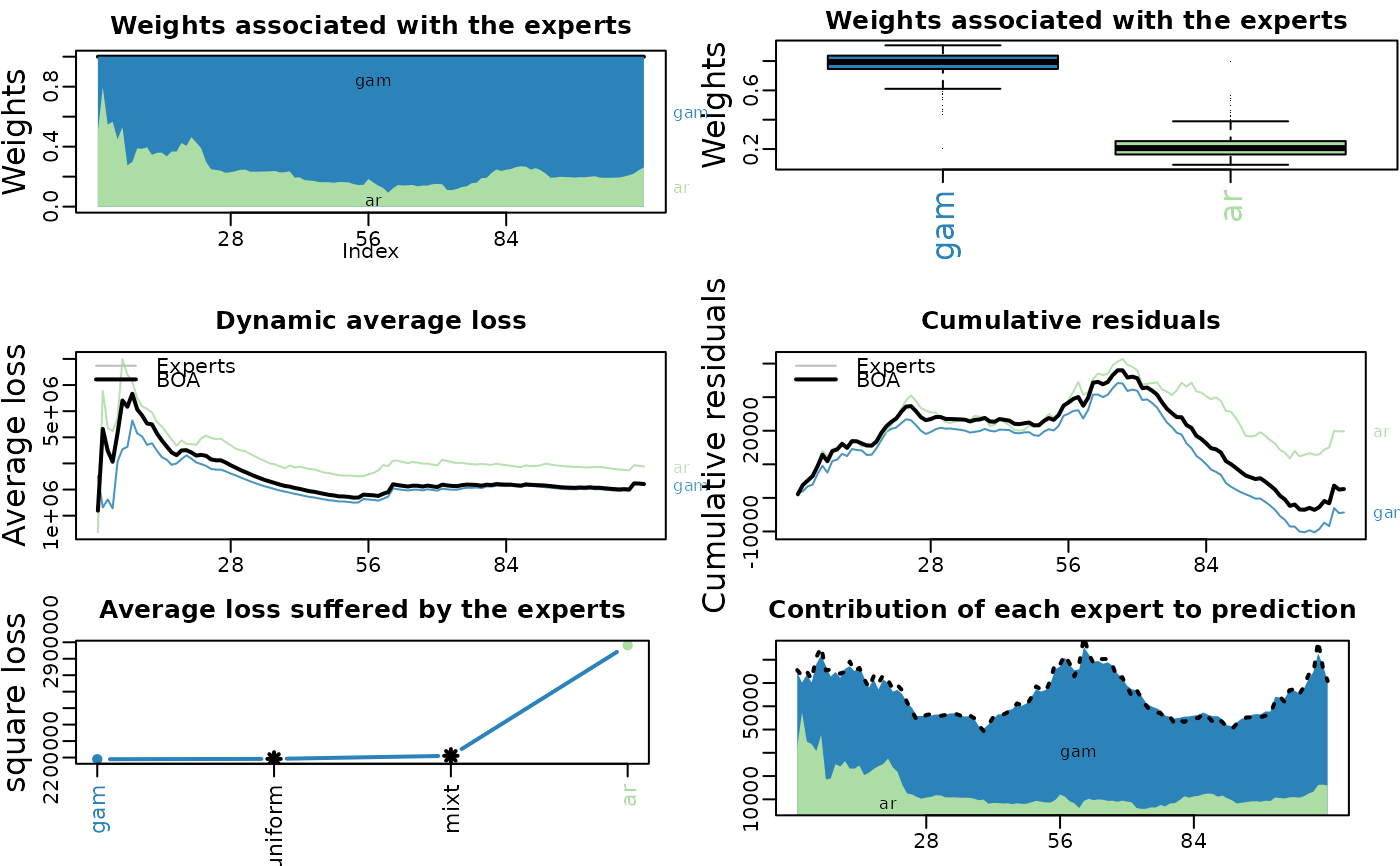
if(interactive()){
plot(m1.BOA)
}
# Plot options
##################################
# ?plot.mixture
# static or dynamic : dynamic = F/T
plot(m1.BOA, dynamic = FALSE)
# How good are the expert? Look at the oracles
oracle.convex <- oracle(Y = Y, experts = X, loss.type = 'square', model = 'convex')
if(interactive()){
plot(oracle.convex)
}
oracle.convex
#> Call:
#> oracle.default(Y = Y, experts = X, model = "convex", loss.type = "square")
#>
#> Coefficients:
#> gam ar
#> 0.751 0.249
#>
#> rmse mape
#> Best expert oracle: 1480 0.0202
#> Uniform combination: 1480 0.0206
#> Best convex oracle: 1450 0.0200
# Is a single expert the best over time ? Are there breaks ?
oracle.shift <- oracle(Y = Y, experts = X, loss.type = 'percentage', model = 'shifting')
if(interactive()){
plot(oracle.shift)
}
oracle.shift
#> Call:
#> oracle.default(Y = Y, experts = X, model = "shifting", loss.type = "percentage")
#>
#> 0 shifts 28 shifts 55 shifts 83 shifts 111 shifts
#> mape: 0.0202 0.0159 0.0154 0.0154 0.0154
# Online aggregation of the experts with BOA
#############################################
# Initialize the aggregation rule
m0.BOA <- mixture(model = 'BOA', loss.type = 'square')
# Perform online prediction using BOA There are 3 equivalent possibilities 1)
# start with an empty model and update the model sequentially
m1.BOA <- m0.BOA
for (i in 1:length(Y)) {
m1.BOA <- predict(m1.BOA, newexperts = X[i, ], newY = Y[i], quiet = TRUE)
}
# 2) perform online prediction directly from the empty model
m2.BOA <- predict(m0.BOA, newexpert = X, newY = Y, online = TRUE, quiet = TRUE)
# 3) perform the online aggregation directly
m3.BOA <- mixture(Y = Y, experts = X, model = 'BOA', loss.type = 'square', quiet = TRUE)
# These predictions are equivalent:
identical(m1.BOA, m2.BOA) # TRUE
#> [1] TRUE
identical(m1.BOA, m3.BOA) # TRUE
#> [1] TRUE
# Display the results
summary(m3.BOA)
#> Aggregation rule: BOA
#> Loss function: squareloss
#> Gradient trick: TRUE
#> Coefficients:
#> gam ar
#> 0.738 0.262
#>
#> Number of experts: 2
#> Number of observations: 112
#> Dimension of the data: 1
#>
#> rmse mape
#> BOA 1490 0.0203
#> Uniform 1480 0.0206
if(interactive()){
plot(m1.BOA)
}
# Plot options
##################################
# ?plot.mixture
# static or dynamic : dynamic = F/T
plot(m1.BOA, dynamic = FALSE)
 # just one plot with custom label ?
# 'plot_weight', 'boxplot_weight', 'dyn_avg_loss',
# 'cumul_res', 'avg_loss', 'contrib'
if(interactive()){
plot(m1.BOA, type = "plot_weight",
main = "Poids", ylab = "Poids", xlab = "Temps" )
}
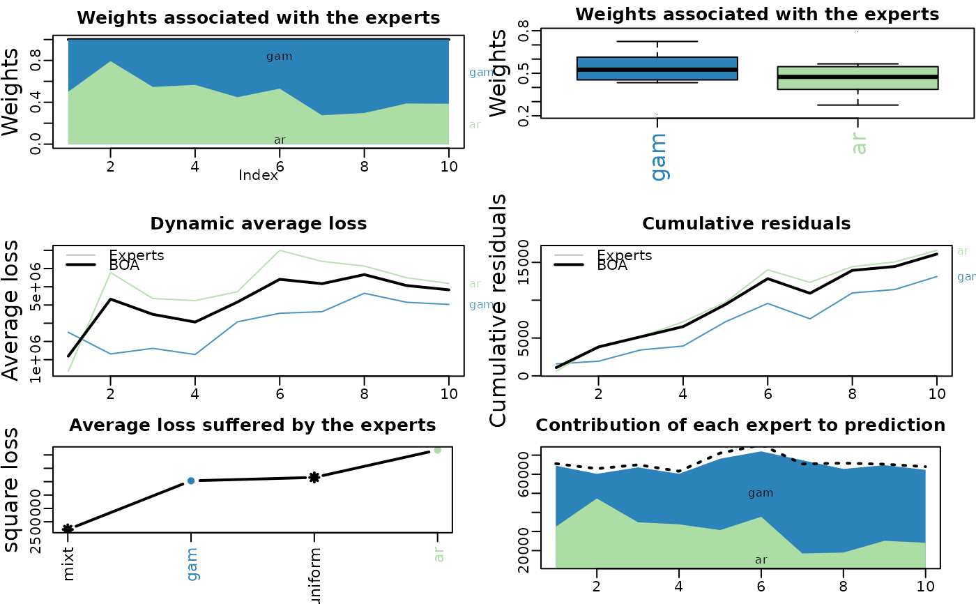
# subset rows / time
plot(m1.BOA, dynamic = FALSE, subset = 1:10)
# just one plot with custom label ?
# 'plot_weight', 'boxplot_weight', 'dyn_avg_loss',
# 'cumul_res', 'avg_loss', 'contrib'
if(interactive()){
plot(m1.BOA, type = "plot_weight",
main = "Poids", ylab = "Poids", xlab = "Temps" )
}
# subset rows / time
plot(m1.BOA, dynamic = FALSE, subset = 1:10)
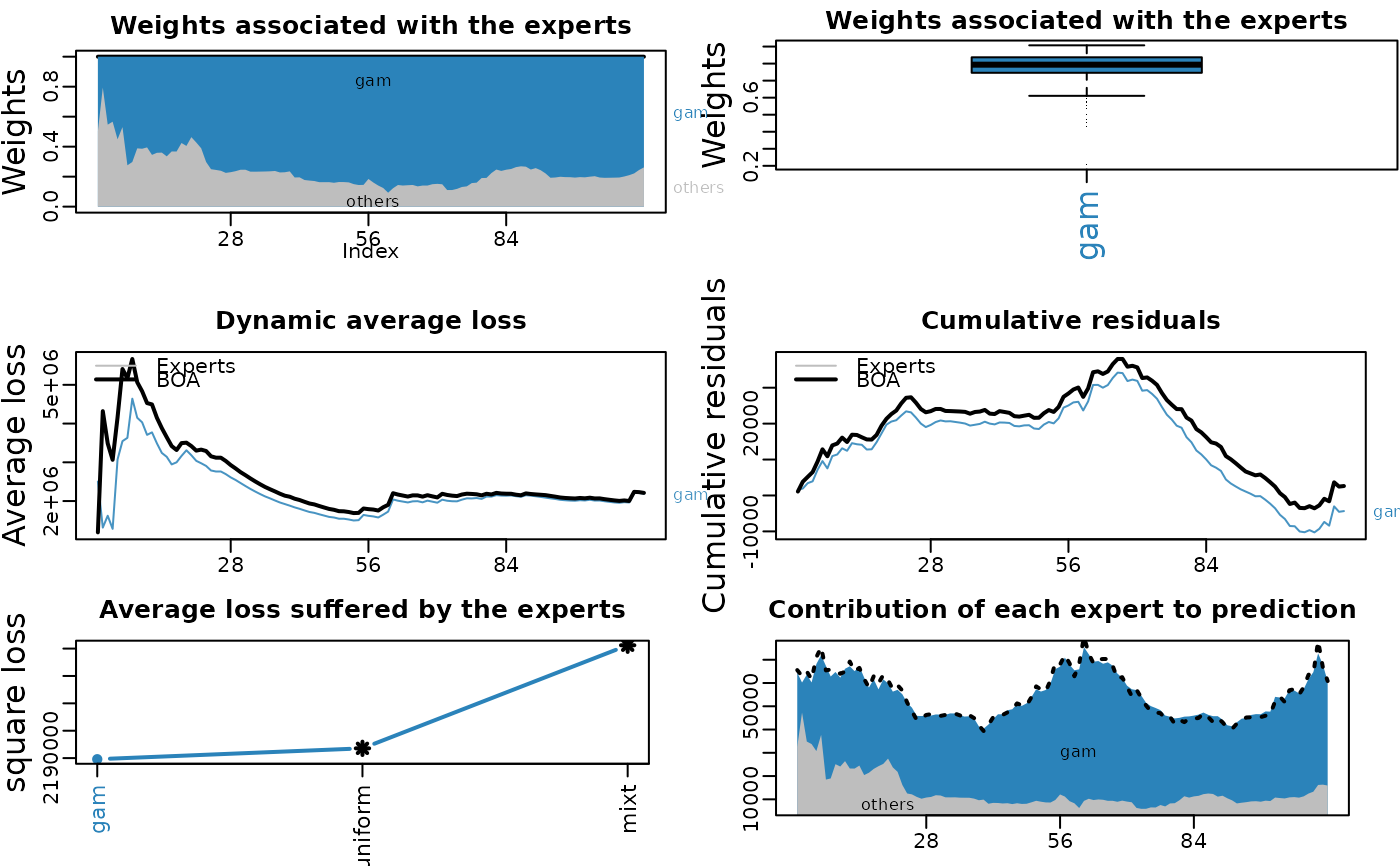
 # plot best n expert
plot(m1.BOA, dynamic = FALSE, max_experts = 1)
# plot best n expert
plot(m1.BOA, dynamic = FALSE, max_experts = 1)
 # Using d-dimensional time-series
##################################
# Consider the above exemple of electricity consumption
# to be predicted every four weeks
YBlock <- seriesToBlock(X = Y, d = 4)
XBlock <- seriesToBlock(X = X, d = 4)
# The four-week-by-four-week predictions can then be obtained
# by directly using the `mixture` function as we did earlier.
MLpolBlock <- mixture(Y = YBlock, experts = XBlock, model = "MLpol", loss.type = "square",
quiet = TRUE)
# The predictions can finally be transformed back to a
# regular one dimensional time-series by using the function `blockToSeries`.
prediction <- blockToSeries(MLpolBlock$prediction)
#### Using the `online = FALSE` option
# Equivalent solution is to use the `online = FALSE` option in the predict function.
# The latter ensures that the model coefficients are not
# updated between the next four weeks to forecast.
MLpolBlock <- mixture(model = "BOA", loss.type = "square")
d = 4
n <- length(Y)/d
for (i in 0:(n-1)) {
idx <- 4*i + 1:4 # next four weeks to be predicted
MLpolBlock <- predict(MLpolBlock, newexperts = X[idx, ], newY = Y[idx], online = FALSE,
quiet = TRUE)
}
print(head(MLpolBlock$weights))
#> [,1] [,2]
#> [1,] 0.5000000 0.5000000
#> [2,] 0.5000000 0.5000000
#> [3,] 0.5000000 0.5000000
#> [4,] 0.5000000 0.5000000
#> [5,] 0.5511391 0.4488609
#> [6,] 0.5511391 0.4488609
# Using d-dimensional time-series
##################################
# Consider the above exemple of electricity consumption
# to be predicted every four weeks
YBlock <- seriesToBlock(X = Y, d = 4)
XBlock <- seriesToBlock(X = X, d = 4)
# The four-week-by-four-week predictions can then be obtained
# by directly using the `mixture` function as we did earlier.
MLpolBlock <- mixture(Y = YBlock, experts = XBlock, model = "MLpol", loss.type = "square",
quiet = TRUE)
# The predictions can finally be transformed back to a
# regular one dimensional time-series by using the function `blockToSeries`.
prediction <- blockToSeries(MLpolBlock$prediction)
#### Using the `online = FALSE` option
# Equivalent solution is to use the `online = FALSE` option in the predict function.
# The latter ensures that the model coefficients are not
# updated between the next four weeks to forecast.
MLpolBlock <- mixture(model = "BOA", loss.type = "square")
d = 4
n <- length(Y)/d
for (i in 0:(n-1)) {
idx <- 4*i + 1:4 # next four weeks to be predicted
MLpolBlock <- predict(MLpolBlock, newexperts = X[idx, ], newY = Y[idx], online = FALSE,
quiet = TRUE)
}
print(head(MLpolBlock$weights))
#> [,1] [,2]
#> [1,] 0.5000000 0.5000000
#> [2,] 0.5000000 0.5000000
#> [3,] 0.5000000 0.5000000
#> [4,] 0.5000000 0.5000000
#> [5,] 0.5511391 0.4488609
#> [6,] 0.5511391 0.4488609